9 minutes
Modelling Technical Debt with Systems Thinking: A Journey from Simple to Sophisticated
Introduction
As an Engineering Director, I’ve long been fascinated by the invisible forces that slow down software teams over time. We call it “technical debt,” but how do we actually model its impact? How do we quantify the cost of shortcuts and make the case for refactoring investment to business stakeholders?
Recently, I discovered Will Larson’s systems thinking tool and thought it might be the perfect way to model technical debt dynamics. What followed was a fascinating learning journey that taught me as much about the fundamental principles of systems thinking as it did about the complex nature of technical debt itself.
In this post, I’ll take you through that exploration—from initial hypothesis to working model, including the dead ends, revelations, and the final insights that emerged. Whether you’re an engineering leader trying to understand systems thinking or someone interested in modelling complex organisational dynamics, I hope this journey provides valuable lessons for your own work.
The Initial Hypothesis
My hypothesis was straightforward: technical debt accumulates when teams take shortcuts under pressure, and this debt creates a “tax” on future development work that compounds over time. This seemed like a perfect fit for systems thinking—stocks (things that accumulate) and flows (rates of change) connected by feedback loops.
I envisioned a model with key components:
- Stocks: TechDebt, Features, FeatureBacklog, TeamProductivity
- Flows: BusinessDemand, FeatureDelivery, DebtAccumulation, DebtPaydown
- Feedback Loops: Higher debt → lower productivity → more pressure → more shortcuts → more debt
Research showed that technical debt creates vicious cycles in organisations, with companies spending 20-40% of their IT budget managing it. This reinforced my belief that systems thinking could help visualise and quantify these dynamics.
Early Attempts and Learning the Tool
Using Will Larson’s systems tool, I started with a basic specification:
TechDebt(0)
Features(100)
Backlog(10)
TeamCapacity(4)
Productivity(0.85)

[BusinessRequests] > Backlog @ 10
Backlog > Features @ Rate(TeamCapacity * Productivity * 0.6)
Features > TechDebt @ Rate(Features * 0.12)
TechDebt > [DebtFixed] @ Rate(TeamCapacity * 0.3 * Productivity)
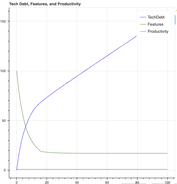
This looked promising—business requests flow into the backlog, the team delivers features (creating some debt), and allocates capacity to fixing debt. Simple and elegant.
But when I ran the simulation, something was missing. The model showed debt accumulating and being paid down, but productivity remained constant at 0.85 throughout the simulation. The whole point—that technical debt slows teams down—wasn’t captured.
The Productivity Challenge
This is where the learning really began. How do you model a variable that should decrease as another variable increases? My initial attempt felt intuitive but was completely wrong:
TechDebt > Productivity @ Leak(0.010)
I expected this to reduce productivity as debt grew. Instead, productivity increased! Through investigation with Perplexity, I discovered a fundamental limitation of my understanding: in the systems tool, Leak(f) moves a fraction of the source to the target—it doesn’t subtract from the target.
My second attempt used Conversion:
Productivity > [LostProductivity] @ Conversion(TechDebt * 0.018)
This technically worked—productivity did decrease as debt grew—but the behaviour was completely unrealistic. For 79 simulation rounds, productivity stayed constant at 0.85, then suddenly collapsed to zero in just a few rounds:
Round 79: Productivity = 0.85
Round 80: Productivity = 0.0
Round 81: Productivity = 0.0
This created a “cliff effect” where everything was fine until catastrophic failure. Looking at 100 rounds of simulation data revealed the core issue: the model showed steady debt accumulation for 80 rounds, constant productivity, then sudden productivity collapse and complete halt in feature delivery.
This isn’t how technical debt works in reality. Real teams experience gradual productivity decline as debt accumulates—not sudden catastrophic failure after a long plateau.
Understanding Systems Thinking Principles
The breakthrough came from deeper research into Donella Meadows’ “Thinking in Systems” and studying Will Larson’s example notebooks more carefully. I discovered several key insights:
1. Not Everything Should Be a Stock
Productivity in systems thinking terms isn’t really a “stock” (something that accumulates)—it’s more like a constraint or capacity modifier. The tool excels at modelling accumulating quantities but struggles with variables that should be functions of other variables.
2. Study the Examples
Larson’s reliability notebook showed sophisticated feedback where Changes > Latent @ Conversion(1 / (1 + Remediated)) - meaning fewer changes create latent issues when remediation is higher. Variables can be functions of other stocks using the Conversion mechanism properly when the relationships are modelled as stock transformations.
3. Priming Is Essential
A critical realisation: in systems thinking, no flow will happen unless the source has at least one unit. If stocks start at zero, the entire system can remain “dead.” Every active stock in a flow chain must be initialised with non-zero values.
The Breakthrough: Rethinking the Problem
Instead of trying to model productivity as a stock that gets depleted, I needed to model it as a capacity constraint on flows:
TechDebt(0)
Features(0)
Backlog(20)
TeamCapacity(20)
ProductiveCapacity(17)    # Start with 85% of team capacity

[BusinessRequests] > Backlog @ 10
Backlog > Features @ Rate(ProductiveCapacity * 0.6)
Features > TechDebt @ Leak(0.12)
TechDebt > [DebtFixed] @ Rate(ProductiveCapacity * 0.3)
ProductiveCapacity > [LostCapacity] @ Conversion(TechDebt * 0.01)
[TeamRegen] > ProductiveCapacity @ Rate(0.8)
This approach:
- Models productivity as capacity constraint on flows rather than a stock
- Uses
Conversionrates that depend on other stocks (following Larson’s examples) - Creates realistic feedback where TechDebt gradually reduces ProductiveCapacity
- Avoids cliff effects through proper system structure
Understanding the Results
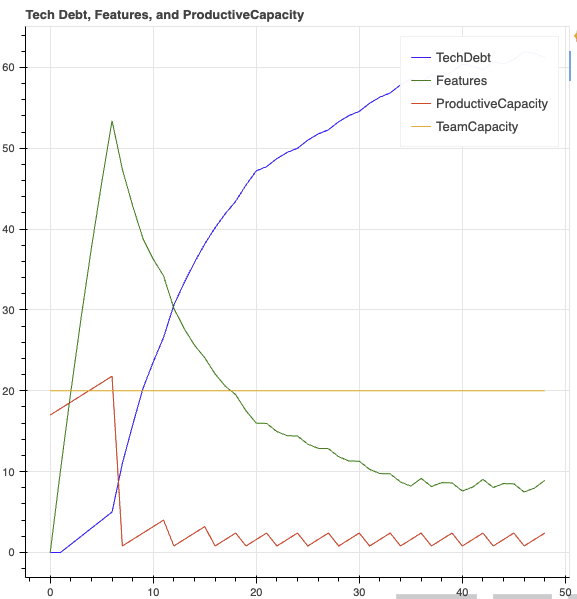
When I ran this model for 48 rounds, the results told a compelling story:
The Dynamics
- Early rounds: Feature delivery ramps up (as ProductiveCapacity is high), quickly accumulating TechDebt
- Feedback kicks in: Rising TechDebt causes ProductiveCapacity decline, throttling new Features
- Vicious cycle: Lower capacity means fewer features delivered, but also less new debt created; however, existing debt continues eroding capability
- Backlog growth: Unchecked demand exceeds constrained delivery capacity
What the Model Shows Us
Looking at the visualisation, we see:
- TechDebt (blue): Steady, almost monotonic increase after initial cycles
- Features (green): Rapid rise to peak, then decline and oscillation, never reaching early peak again
- ProductiveCapacity (red): Sharp decline after initial plateau, then oscillation between low values and brief recoveries
- TeamCapacity (yellow): Constant baseline, as modelled
This captures the essential dynamic: building up technical debt restricts future throughput and creates negative feedback loops.
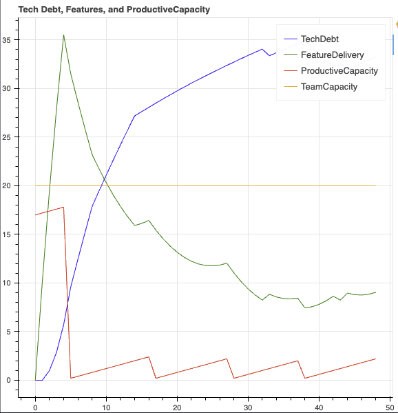
Making the Model More Realistic
The initial results, while demonstrating the core dynamics, showed some unrealistic behaviour—particularly the “sawtooth” pattern in ProductiveCapacity. Through iteration, I identified several improvements:
1. Smoother Capacity Erosion
ProductiveCapacity > [LostCapacity] @ Conversion(TechDebt * 0.015)
Increased the erosion rate to make capacity decline more responsive to debt accumulation.
2. Adaptive Debt Paydown
TechDebt > [DebtFixed] @ Rate(ProductiveCapacity * 0.3 + TechDebt * 0.02)
Added a component that increases debt payment as debt grows, modelling organisational “crisis response.”
3. Reduced Regeneration
[TeamRegen] > ProductiveCapacity @ Rate(0.2)
Lowered the regeneration rate to prevent unrealistic capacity spikes.
These changes produced more realistic, continuous decline in ProductiveCapacity rather than sharp oscillations.
Key Lessons Learned
1. Systems Thinking ≠ Systems Tools
Systems thinking is a mental model and approach to understanding complex problems. Systems modelling tools are just one way to explore these ideas. Don’t confuse the concept with any particular implementation.
2. Understanding Tool Constraints
Every modelling tool is optimised for certain types of problems. The systems tool excels at:
- Accumulating quantities (features delivered, debt principal)
- Constant or simple variable rates
- Physical flows and constraints
- Basic feedback loops
It struggles with:
- Variables that should be functions of other variables
- Non-linear relationships
- Immediate dependency relationships
- Complex conditional logic
3. Model Structure Matters More Than Parameters
The biggest insights came from changing how I structured the model, not just tuning parameters. Treating productivity as capacity constraint rather than depleting stock was the key breakthrough.
4. Stocks vs. Flows vs. Constraints
In Donella Meadows’ framework:
- Stocks are things that accumulate (technical debt, features delivered)
- Flows are rates of change (feature delivery rate, debt accumulation rate)
- Constraints limit flows (team capacity, productivity)
Understanding these distinctions is crucial for effective modelling.
5. Start Simple, Add Complexity Gradually
Begin with the minimal viable model that captures core dynamics, then layer on complexity. Each addition should serve a clear purpose in making the model more realistic or insightful.
What the Model Teaches Us About Technical Debt
Beyond the technical learning, the model reveals important insights about managing technical debt:
1. The Compound Nature of Technical Debt
The model clearly shows how technical debt doesn’t just slow current work—it reduces the team’s capacity for all future work, creating compound effects over time.
2. The Importance of Proactive Investment
Small, consistent investment in debt reduction (represented by the debt paydown flow) can prevent catastrophic productivity collapse. The model shows that waiting too long makes recovery much more difficult.
3. The Business Case for Refactoring
By quantifying how productivity constraints compound over time, the model provides a framework for making business cases for refactoring investment. The cost of inaction becomes visible.
4. Equilibrium Points Matter
The model helps identify sustainable equilibrium points between feature delivery and debt management. Pure feature focus leads to productivity collapse; too much refactoring focus leaves business needs unmet.
Conclusion
This exploration taught me that modelling technical debt requires understanding both the domain and the fundamental principles of the modelling approach. While Will Larson’s systems tool has limitations, it provided valuable insights into stock-and-flow dynamics and feedback loops.
The real value wasn’t just in the final model—it was in the journey of discovery. Struggling with the tool’s limitations forced me to think more clearly about the nature of technical debt, productivity, and the feedback loops that govern software development.
For engineering leaders interested in systems thinking, I’d recommend:
- Start with simple models to understand basic dynamics
- Embrace the limitations of your chosen tools—they often teach you as much as the capabilities
- Focus on structure over parameters—how you model relationships matters more than precise values
- Study examples from practitioners who’ve used the tools successfully
- Share your models with your team to build shared understanding
The goal isn’t to predict the future with mathematical precision—it’s to create shared mental models that help teams make better decisions about technical debt, refactoring investment, and long-term system health.
Whether you use systems thinking tools, spreadsheets, or just conceptual models, the key is making invisible dynamics visible and creating a common language for discussing the long-term costs of technical decisions.
Systems thinking has given me a more nuanced understanding of the forces at play in software development. The technical debt model is just one example—the principles apply to hiring, incident response, team scaling, and countless other engineering challenges we face.
The next time you’re grappling with a complex organisational dynamic, consider whether systems thinking might help you see the underlying structure more clearly. Sometimes the most profound insights come not from the final model, but from the journey of building it.
References and Further Reading
Throughout this exploration, I referenced several key resources:
- Project Repo - My Github with the project files to follow along
- Will Larson’s systems tool - The primary modelling tool explored
- Donella Meadows’ “Thinking in Systems” - Foundational systems thinking principles
- Will Larson’s reliability notebook example - Sophisticated feedback loop implementation
- Systems thinking leverage points - Understanding where to intervene in systems
The complete model specifications and analysis from this exploration provide a practical starting point for engineering leaders interested in systems thinking approaches to technical debt management.